Khanh's Gallery

When we look up at the night sky, we are often tricked by the illusion of stillness. The stars appear as fixed, unblinking points of light—eternal and unchanging. But if we could look with the eyes of a spectroscope, the silence would vanish. We would see a universe that is roaring, spinning, and violently expanding.

Nowhere is this dynamic nature more elegant than in the spectral signature known as the P Cygni profile. It is a curve on a graph, yes, but it is also a portrait of a star in the act of breathing.

The Signature of a Restless Star

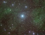
To the casual observer, 34 Cygni (P Cygni) is a faint star in the constellation of the Swan. But to the astrophysicist, it is a legend. In 1600, it flared up suddenly, catching the attention of astronomers like Willem Janszoon Blaeu, before fading and fluctuating over centuries. It was not a supernova, but a star so massive and unstable that it was struggling to hold itself together.

P cygni is a hypergiant luminous variable (LBV) star of spectral type B1Ia+ in the constellation of Cygnus. It is well-studied as its spectrum exhibits a distinctive spectroscopic feature known as a P Cygni profile, where both absorption and emission is present in the profile of the same spectral line. this indicates the presence of a gaseous shell rapidly expanding away from the star, and is suggestive of rapid mass loss from a dense stellar wind.

The Interplay: Geometry and the Doppler Effect

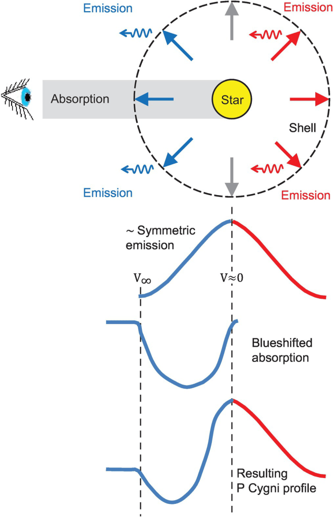
The beauty of the P Cygni profile lies in its geometry. It is a perfect example of how our perspective—our location as the observer—dictates what we see.

Imagine a massive star surrounded by a shell of gas that is expanding outward in all directions.

1. The Blue Valley (Approach): The gas directly between us and the star is rushing toward us. Because of the Doppler effect, the light this gas absorbs is shifted to shorter, bluer wavelengths. This creates the absorption trough on the left side of the profile. This “blue edge” is critical; by measuring how far it shifts, we can calculate the terminal velocity of the wind—often thousands of kilometers per second.
2. The Red Peak (Departure): The gas surrounding the star is also glowing. But because the shell is expanding spherically, the lobes of gas moving away from us (or to the sides) emit light that is Doppler-shifted to the red or stays central. This creates the emission peak.

Together, they form a complete picture of motion. We are not just seeing “gas”; we are seeing the geometry of an explosion frozen in time.

Calculation

Set up Coordinate and the Doppler Shift

To understand the spectral line shape, we model the star as a central source of continuum light with radius $R_*$, surrounded by a spherical shell of gas extending to a radius $R_\text{shell}$. This shell expands radially outward with a constant terminal velocity, $v_\infty$.

We need to define the coordinate system where the $z$-axis points toward the observer. We then have:

• Radial vector: Any packet of gas at position $(r, \theta, \phi)$ moves with the vector $\mathbf{v}=v_\infty \bold{\hat{r}}$.
• Line of sight (LOS) velocity: The observer only detects the component of velocity projected onto the $z$-axis $(v_\text{obs}=v_z)$.

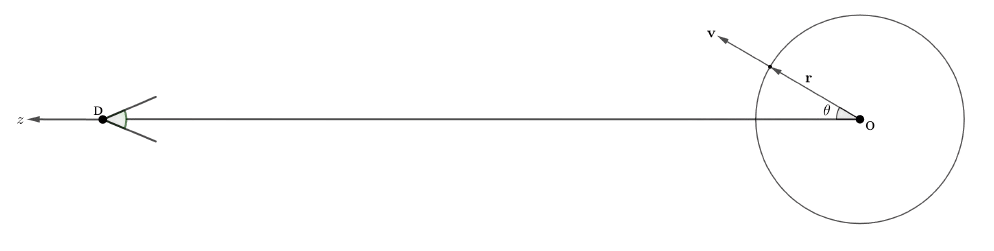
Using the angle $\theta$ (the angle between the line of sight and the radial vector), the velocity observed is:

Note: The negative sign indicates motion towards the observer when $0^\circ\le \theta\le 180^\circ.$

The wavelength shift $\Delta \lambda$ observed for any packet of gas is given by the non-relativistic Doppler formula:

This equation maps the geometry of the shell directly to the wavelength axis of the spectrum.

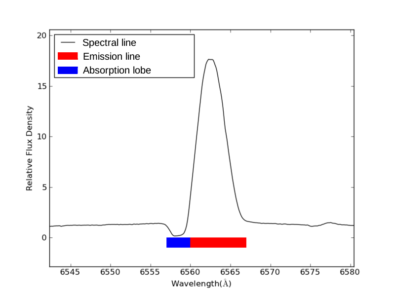
P Cygni Profile

The P Cygni profile is the superposition of two distinct physical regions: the Emission Lobe and the Absorption Column.

The Emission Component

The expanding shell is optically thin to continuum radiation but optically thick to the line transition. It emits light in all directions.

• Blue-shifted Emission: Comes from the front hemisphere of the shell $0^\circ\le \theta\le 90^\circ$, excluding the column directly in front of the star.
• Red-shifted Emission: Comes from the back hemisphere $90^\circ\le \theta\le 180^\circ$. Note that the region directly behind the star (the “occulted zone”) is blocked, slightly reducing the red peak, though this effect is often negligible if $R_\text{shell} \gg R_*$.

Because the shell emits at all angles $\theta$, the emission line is broadened into a “flat-topped” or parabolic shape spanning from $-v_\infty$ to $+v_\infty$.

The Absorption Component

This is the defining feature. Absorption only occurs where the cold wind lies between the observer and the hot stellar surface. This region is a narrow cylinder directly along the line of sight ($z$-axis) where $\theta\approx0$. Therefore, in this region, $\cos\theta\approx 1$, and the gas is moving directly toward us at maximum speed $v_\infty$. This creates a sharp absorption trough centered at the maximum blue-shift:

The “Blue Edge” Diagnosis

In professional astrophysics, the most critical measurement is the “Blue Edge” of the absorption trough. This point represents the fastest-moving material in the wind.

We can calculate the terminal velocity of the stellar wind ($v_\infty$) directly from the spectrum by measuring the wavelength at the bluest edge of the absorption dip $(\lambda_\text{edge})$:

DIY Astrophysics: Calculate the Wind Speed

Want to measure the speed of a star’s “breath” yourself? You can use this simple Python script to calculate the terminal velocity of a stellar wind using real spectral data.

def calculate_wind_velocity(rest_wavelength, blue_edge_wavelength):
    """
    Calculates the terminal velocity of a stellar wind based on the 
    P Cygni profile absorption edge.
    """
    c = 299792.458 # Speed of light in km/s
    
    # Calculate the shift
    delta_lambda = rest_wavelength - blue_edge_wavelength
    
    # Apply Doppler formula
    velocity = c * (delta_lambda / rest_wavelength)
    
    return velocity
# --- EXAMPLE: P Cygni's Hydrogen-Alpha line ---
# Rest wavelength: 6562.8 Angstroms
# Observed blue edge: 6558.7 Angstroms
wind_speed = calculate_wind_velocity(6562.8, 6558.7)
print(f"The stellar wind is moving at: {wind_speed:.2f} km/s")

Conclusion

We often get lost in the rigidity of calculations, treating stars and galaxies as static data points to be solved. But the real philosophy of this science—and the core of my approach—lies in the interplay. It is about looking past the isolated variables to see the dynamic, evolving ecosystem they inhabit.

Take P Cygni, for instance. To the untrained eye, it might just be a point of light or a specific spectral curve. But from that single snapshot, we can infer the entire turbulent reality of a Luminous Blue Variable (LBV) star. We see the violent stellar winds driving mass loss; we see a star at the very limit of stability, fighting against its own radiation pressure.

The math gives us the specific numbers of that expansion, but it is the physical intuition that allows us to construct the full story from a single piece of evidence. The most important understanding isn’t the precise calculation of the wind speed, but grasping the ‘bigger picture’—the chaotic, beautiful interplay of forces that drives the universe’s evolution.